Results & Findings
- Langevin Dynamics:
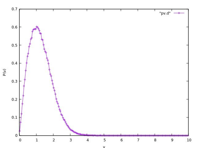
Think of it like driving a car, but the road’s full of potholes and unpredictable speed bumps. Langevin dynamics lets us simulate the motion of our polymer while factoring in all the random bumps from the environment and the constant friction from the medium it’s in. We’re talking random noise and forces that make sure our polymer doesn’t just sit there like a lump. It moves, it fluctuates, it’s alive.
- Brownian Dynamics:
Now, Brownian dynamics takes things down a notch – the polymer just goes on a random walk, driven by all the invisible particles around it. No superpowers, just collisions and random movements, much like that random walk at 2 a.m. after a coffee bender. It’s messy, but it’s how particles behave in a solvent, and that’s what we need to understand for this project.
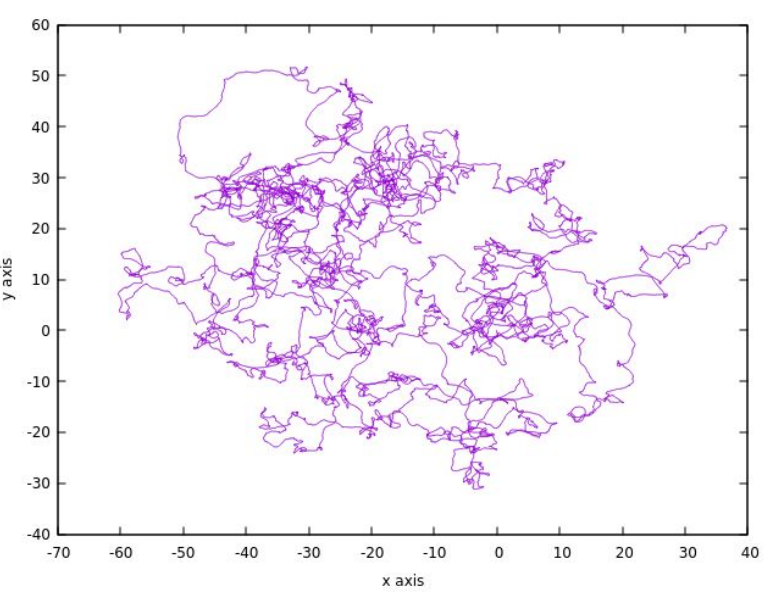
The code? We wrote it from scratch in Fortran. None of that pre-packaged stuff – we’re
taking this bad boy down to the metal, baby. And for the visuals, we fire up MATLAB.
Plot those graphs, show those transitions, and make sure we can visualize every step
in the transition from coil to globule.